|
|
 |
a VB5 program for Windows95/98 ©1999-2002andykidd |
An Introduction to OTAeXplorer | to top |
The main purpose of OTAeXplorer is to aid in determining optimal ocular sets
for any particular OTA.
The program uses calculation of M', Mr and M", which are:
|
Of particular interest, Mr, the magnification of resolution, is the magnification required to make the resolution present at the focal
plane visible to the [average?] human eye. In other words, employing a magnification
greater than Mr will make an image larger but it will not [in theory] normally reveal any more detail.
Because of differences in visual acuity among individuals [and age groups!] this is probably an overly-optimistic value. The particular subject being observed has a bearing on this as well. On point-source objects, as when splitting doubles, for instance, one will generally need and want much greater magnification than Mr [on the order of 2 to 3 times more]. Planetary observation on nights of good seeing will also benefit from more magnification.
While this Mr magnification may seem limited in value, i've personally found that with most OTAs it will generate a great balance between visible detail and sharpness, light scavenging and FOV for observing DSOs and general star-grazing. Interestingly, this Mr value will give right around a 2mm exit pupil and i don't know if there is any significance to this.
Though using an ocular with an OTA that developes a magnification different than the Mr for that OTA is perfectly acceptable and practiced and not to mention often desireable, in theory at least, one would be wasting either light or resolving power which of course may not necessarily be a problem, depending
on the circumstances at the time. In any case it is something to keep in mind.
Though these values: M', Mr and M" are not entirely empirical, as they do have a mathematical basis in theory, OTAeXplorer uses a three mode system for determining them depending upon how concerned the user is about the theoretical values or how far the user wishes to 'push' his OTA. As with Dawes criterion for maximum resolution, there is often times some apparent disagreement between theory and observations in practice. The settings available in OTAeXplorer from the 'Radical' to 'Conservative' functions represents the range generally accepted as describing reasonable values. The Mr function remains unchanged and is based on Dawes' empirical criterion as the small amount of extra magnification [as opposed to the theoretical value] would not affect the value of this function significantly.
To help make OTAeXplorer quick to use, it contains user updateable 'databases' and 'catalogs' that allow you to quickly store and retrieve the necessary parameters for oculars and OTAs required by the program.
The program comes with pre-configured 'catalogs' of numerous OTAs and hoardes of eyepieces and barlows from many common manufacturers. If you don't see equipment listed in these included catalogs, don't fret; as previously mentioned the catalogs are createable and updateable by the user.
The output can be displayed in the form of either a chart or graph to help aid in the 'digestion' of the data.
The following instructions will explain in further detail how to use these features.
Note: throughout these instructions, the word 'ocular' is used to mean 'eyepiece', which in debate may or may not be actually technically 'accurate' but it's done here because:
1) i think it's a really cool word
b) 'ocular' is so much easier to type than 'eyepiece' [especially since i don't have to mentally recite 'i before e...' when i type it].
p.s. i know the last point could be remedied by using the common abbreviation EP, and probably will do that in future 'incarnations' of the program just to be 'up to date', but i still prescibe to #1 listed above
The Main Program Window | to top |
|
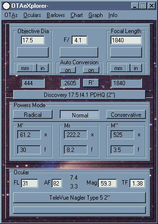
Below you see the OTAeXplorer Main Program Window with some sample values. Starting at the top, you'll see the menu bar with selections for the OTA and Ocular databases as well as for the Chart and Graph displays. Default values can be changed by the 'Setup' selection in the 'Info' drop-down menu that's on this main menu bar.
The Objective Dia and Focal Length boxes each contain an input parameter window. This is where you manually enter those parameters. The buttons below the input windows perform the calculation function for that parameter. OTAeXplorer will calculate any of the three main parametes (including the f/ value) from any other two parameters entered. Below the calculation button for these parameters is a 'mm/in' button which has two functional uses. The first function mode is to select whether the input parameter box displays in millimeter or inch values. The little button between unselects both buttons. The use of these button arrays will [may!] become clearer in the next section that cover the 'auto conversion' function.
IMPORTANT NOTE: If you use a device such as a focal reducer for a SCT or Paracorr for a short f-ratio scope you'll want to pay attention to the special feature subsection of the database section when you get there.
Between the OD and FL input boxes is the f/ input box with it's calculation button below. When using the database and catalogs, the OD and FL are supplied so this f/ calculation button is the one you'd be using to run the calculation function. |
|
Between the OTA section and the M section is a combination OTA 'Descriptor Label' and 'Calculate/Clear' button. This will display the name of the OTA sent from the database [if there is one] and will perform a 'smart calculate' function on the OTA data. This 'smart calc' function will calculate or recalculate the OTA specs [based on which parameters are the most recently changed] and will more or less serve the same function as the 'dedicated' calculate buttons below the individual OTA parameters. If using this button doesn't calculate the parameter wanted then you'll have to select one of the specific parameter calculation buttons. A right-click on this button will clear the OTA parameter fields.
As you can see, some of these buttons on the MPW are actually 'labeled' only with the 'tool-tips' which can be disabled.
Below the Calc/Clear button is the 'M' displays. Listed here are the power in magnification and corresponding ocular focal length for that power with the given OTA as discussed in the intro. The values can be expressed in one of three different 'modes', depending on how 'radical' or 'conservative' you want OTAeXplorer to be while computing them. The mode OTAeXplorer starts in is also selectable through the 'Setup' function that was mentioned above.
The last section of the Main Program window has an Ocular Calculator that will compute the magnification and true field an ocular will give you with the OTA. This function can be used 'backwards, forwards and inside-out' so to speak.
If you want to determine, for instance, what ocular focal length and apparent field you need to get a particular magnification and true field, just enter those values and OTAeXplorer will give it to you with a click of the [tool-tip labeled] calculate button just below the calculator's parameter boxes [this button also serves as the Ocular Descriptor label if one has been sent from a Ocular database]. If OTAeXplorer doesn't seem to want to compute the right value, you can sometimes 'force' it to by 'highlighting' the value you want it to keep by clicking on that value's label. When a 'keeper' value is selected, it's label will turn light. Note that any parameter changed is automatically a 'keeper'. If OTAeXplorer refuses to calculate a particular parameter or from those you have specified, it probably can't be done.
The values displayed between the 'AF' and 'Mag' boxes are, from top to bottom, the exit pupil size and magnification per inch of aperture that ocular will develop with the particular OTA.
A shifted right-click on the 'TF' label will activate the Drift Time function and two boxes will appear on the ocular calc button. If you enter the 0 declination drift-time in minutes [left box] and seconds [right box] determined experimentally from an ocular of this FL, OTAeXplorer will automatically calculate the actual true field of view you are getting with that ocular [the 'true true field of view' if you want to call it that. I guess that could be refered to as the T2FOV?].
On the bottom of the MPW is a 'clear' button. Left-clicking this button will clear both the OTA and Ocular sections. A right-click will clear only the Ocular section. |
The Databases and Catalogs | to top |
Right-clicking on the Database icon in the lower right corner of the database window will allow you to cycle through the three OTA, Ocular and Barlow bases. Clicking on this icon will change to the database that the icon is displaying.
See 'Advanced Database Functioning' for more info on how to use the databases.
The Ocular and Barlow databases have additional filebases linked to the OTAs. A click on the label above the database icon (or clicking the 'OTA' function in the drop-down file menu] will select between the 'global' and 'OTA specific' filebases [when a OTA has been 'selected' by 'Send'ing it to the main program window]. By using this control, an additional full array of filebases that are linked to each specific OTA in any and all of the three OTA filebases are available for use.
Selecting an OTA or Ocular in the file list by clicking on it and then clicking the 'Send' button will transfer that data to the Main Program Window for use in calculations. Doing the same on a Barlow filebase sends the Barlow to the Chart/Graph function for use in those calculations [the MPW Ocular Calculator has no provision for utilizing barlow devices at this time].
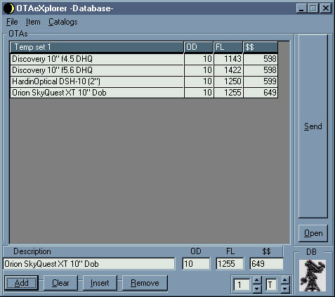 |
The input boxes at the bottom of the window are used to manually enter items into the filebase. It's as simple as entering your data into the boxes or 'Send'ing the information from a catalog and clicking on the Add button. You will, of course, have to click Save in the File menu to make any changes permanent. Other buttons are included for clearing the input boxes as well as inserting the data to a selected point in the filebase and removing a selected item. Removing a selected item will transfer that items data to the data input boxes [unless the boxes corresponding label is 'highlighted' by a right-click on the label]. Selecting more than one item [by a click-drag] will actually erase that data without transfering any of it to the data input boxes. Some additional editing functions include double-clicking an item in the list will place that items data into the input boxes without actually removing the item from the list as the 'Remove' button does with a single item selected. Entry fields that have been 'locked' [by right-clicking on an entry box label, which will then become highlighted] will not be 'overwritten'. A click on an input box's label will clear that input box [the exception is in the catalog windows where this will only always clear the data field when the label is not in it's 'highlighted' or locked mode for the search function. 'Locked' entry windows can be cleared with a shifted click]. |
|
While OTAeXplorer does come with an assortment of Catalogs, it does not come with any of the filebases preconfigured for Oculars, OTAs or Barlows. These databases are intended to be 'populated' with equipment either 'manually, or by 'Send'ing from a Catalog by the user.
|
A SPECIAL FEATURE of the Barlow database is an 'ALT'ternate 'Send' function.
The Chart and Graph modes can incorporate a focal length-altering device into all calculations by holding the 'Alt' key down when 'Send'ing it. Doing this will cause that device's magnification value to be 'stacked' with all the oculars used for a chart or graph display and affect all computations in these modes. If you include any things that affect the OTA's focal length such as a focal reducer for a SCT or a Paracorr for a short-focus scope into the barlow database, you can cause one of them to be included for all the calculations in those modes without taking up one of the two available spots in the Barlow function by 'Alt-Sending' them in this way. This device can be removed from the calculations when in Chart and Graph modes by holding down the 'Alt' key and clicking on the 'clear' button in the 'Barlow' section of those mode windows.
OTAeXplorer Catalogs make it easy to populate your database with OTAs, Oculars and Barlow lenses...
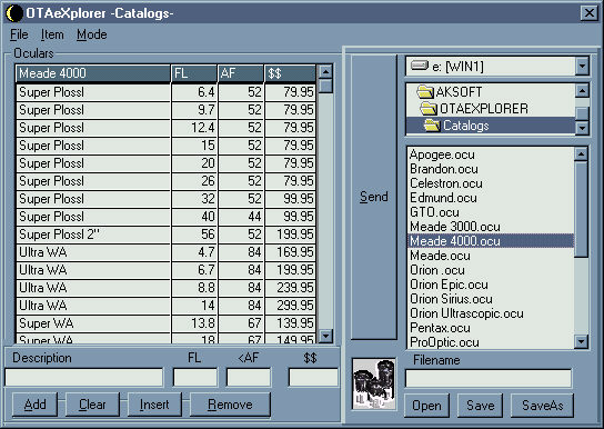
The Catalogs are very similar to and mostly used the same way as the databases, with a few exceptions.
The 'Send' button for the catalog windows transfers the selected data to the data input boxes of the appropriate database window instead of the MPW as the database 'Send' button does.
Unlike the files of the databases, the catalog files are and need to be named by the user when they are created. Controls are included in the catalog windows to select catalogs and create new ones.
Note: if you include a hyphen [ - ] in the catalog name, the hyphen and anything beyond it in the catalog name will not show up in the equipment description for any component used from that catalog.
|
There is the addition of the File listbox for selecting the files (and directory and drive if necessary). In this way you can append or even create your own catalogs for use with OTAeXplorer.
To create a catalog just add your items to the catalog data grid and enter the filename you wish to save it under in the filename input box and click the 'SaveAs' button. No file extension is necessary as OTAeXplorer will add it for you automatically. |
|
ADF is a little different for the Ocular and Barlow databases than it is for the OTA databases. As mentioned previously, while there is only one 'set' of these filebases for OTAs [9 bases in each of the three 'Main' , 'Alt' and 'Temp' filebases] there are available the same array of additional bases in the Ocular and Barlow databases that are 'linked' to each OTA in any and all of the OTA filebases.
What this amounts to, is different lists of OTAs, Oculars and Barlow lenses can be stored in each of their corresponding 'Main', 'Alt' and 'Temp' filebases and different lists of Oculars and Barlows can be stored in whole sets of seperate filebases linked to specific OTAs in the OTA filebases that compromise the OTA database.
One thing to keep in mind when using the OTA-specific Ocular and Barlow filebases is that the linking is not sophisticated; the links to the OTA database are created when they are saved and this link is to the currently 'sent' [to the MPW] OTA and this link is related to the OTAs position in the OTA filebase the OTA was 'sent' from. Important to note is that these links do not automatically 'refresh' as changes are made to the OTA filebases This may limit their usefulness if your OTA databases are used very 'dynamically', however there is a built-in simple copy function for moving filebases within a database.
To use this copy function, 'Open' the filebase you which to copy and select the 'Copy' and then the 'This' items in the database window's drop-down 'File' menu. Now go to the filebase where you want the 'This'ed filebase copied to and select the 'Here' function in the 'File' menu's 'Copy' section and select whether you want to 'Append' to or 'Replace' the items. Note that in electing 'Replace', the existing filebase that is diplayed on the database's filebase data grid will be overwritten by the 'This' filebase and once the 'Here' filebase is saved it will be completely overwritten by what is now presently being displayed on the database's filebase data grid.
As explained earlier, it is possible to create these additional bases by using the Data Filebase control at the bottom fo the window towards the right. The filebase controls in the drop-down 'File' menu only select between the the 3 'Main', 'Alt' and 'Temp' filebases and whether the 'global' or OTA 'private' filebases are being selected, not which of the 9 individual bases themselves is being used.
Note: In case you need to manipulate or alter a file 'manually', you can see what file in the 'Data' folder you have listed on the database grid by an 'Alt-right-click' on the database icon. This will turn on a box that displays the filebase's actual filename.
All this may sound terribly overcomplicated but it's not that difficult to use in practice once you get used to the ideas. Even though having the databases set up this way limits their versatility somewhat, it's done this way to make the normal file operations quick to use and user-transparent by not having to be constantly weeding through and selecting among myriad files.
Starting with ver. 1.8.xxx, OTAeXplorer will now accomodate zoom oculars. To specify an ocular as a zoom in the catalogs and databases, just seperate the extreme focal lengths and apparent fields of the zoom ocular with the 'tilde' character ~ [i.e. 7~21 for the FL box and 60~40 for the AF box]. In the chart and graph modes, zoom oculars are actually treated as two separate oculars, as one each of the lower and upper limits specified in the ocular FL and AF description.
|
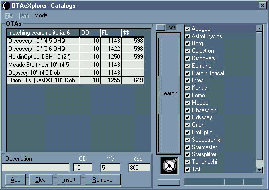
Highlight parameters to search for by a right-click on the corresponding parameter label above the box. Shifting and continuing to right-click will cycle through the search options for that parameter [ 'less than', 'greater than' and 'approximately' ]. No 'prefix' selected will search for that parameter within the standard default tolerance 'window' used by OTAeXplorer which are adjustable through the 'Mode' drop-down menu.
Using a 'prefixed' parameter will alter the standard tolerances. In the 'approximately' mode the tolerance window will be increased by 50%. In 'less than' and 'greater than' modes, the remaining search window tolerance [the upper threshold limit in the case of 'less than' and the lower limit in the case of 'greater than'] will be reduced by 50%. |
|
Catalogs to search through are selectable in the catalog list on the right side of the window. By default all catalogs are selected to search. Clicking on a catalog will select or unselect that catalog. A right-click on this window will 'toggle' all the checks [if you want to search only a couple or few catalogs, 'unselect' the catalogs you want then right-click to 'toggle' the checked catalogs. This is of course faster than 'unselecting' a bunch of catalogs]. A shifted right-click will clear all the check marks. Once your search parameters are set and the catalogs you want to search are selected then click the big 'Search' button and OTAeXplorer will do the rest! |
|
The Chart and Graph Displays | to top |
Now for the cool stuff...
OTAeXplorer can display your Ocular database and selected OTA in two different modes: Chart mode and Graph mode. The Oculars used for the Chart and Graph mode will be last selected Ocular filebase and the values will be extracted from the saved version of that filebase.
Below are some sample charts and graphs i worked up, simulating selection of equipment [not that i can begin to afford a 17.5" dob... just to give you an idea of what OTAeXplorer is capable of displaying; i can still dream, though].
The image below shows the sample data displayed in Chart mode.
Up to two Barlow powers, as you can see, can be computed by clicking on one of the four [programmable] barlow power buttons or by 'Send'ing from the Barlow database. The buttons labeled 's' by the barlow value windows will 'stack' the two barlows together, the computational 'side' of which is controlled by which of the buttons is actived. Disable the 'stack' function by a click on the Barlow frame label or by double-clicking the 's'tack button itself.
To remove barlows from the calculations, click on the 'Clear' button to remove the barlows in reverse order they were added. If you hold the 'Shift' key while clicking the 'Clear' button, the right barlow will be moved to the left position. The 'Clear' button will have to be clicked normally to then actually clear the right barlow position.
The Chart automatically calculates when the Chart window opens using the OTA data from the Maim Program Window and the Ocular database that was active [last selected]. A click on the chart will re-computes the data in the event you want to make any changes to the sort of the oculars, barlow factors [including 'stacking' or 'unstacking' barlows] or duplication factor.
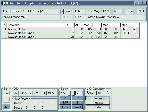 |
The 'D'evice button on the right side of the OTA name box is for the 'FL Device' function. See the special feature subsection of the database section for more information on this.
The Magnifications display at the bottom of the chart lists both the total number of 'unique' and 'duplicated' magnifications available with the particular ocular(s) and barlow(s) configurations. |
In the 'U/D Calculation' box are controls for the 'unique/duped mag' function. The numeric value can be changed directly in the box or by default in the 'Setup' window. After a change to the numeric value has been made, click on one of the factor-type buttons to set the new value and re-calc the chart [a click on chart will cause it to do this]. Three [default selectable] factor types are available and control whether the calculation uses the factor as a percent, absolute magnification value or ratio of x / factor-value.
WHEW... and if all this SO FAR isn't enough for you, read on... there's more because-
You may like 'Graph mode' better!
Below is graph of the same data as in the above chart.
As mentioned above, along with the barlow powers, in both chart and graph mode, the other parameters for sort [in chart mode] and configuration [in graph mode] are saved. To access these different configuration modes you'll need to click on the 'Select' button. Right-clicking on the barlow frame label will toggle between [barlow] 'program' mode and [presets/colors] 'save' mode. When in 'save presets/colors' mode, the button that normally reads 'clear' can be toggled between 'save' and 'recall' functions for storing or retrieving saved setups respectively by right-clicking on it or the [now labeled] 'Set' button. All the graph parameters are saved as a 'configuration'.
In 'presets/colors' Save mode, in addition to the default configuration and the first configuration saved by clicking on the 'Save' button, up to 4 more configurations can be independently saved by clicking on one of the four barlow power boxes [instead of the actual 'Save' button] when the 'Save' button is active. To save these additional configurations, you want to have the barlow power program function inactive by right-clicking on the 'Barlow X' frame label so it reads 'presets/colors' for this save mode. A right-click on the 'Set' button or the 'Save/Recall' button itself will toggle the function between save and recall modes for storing and retrieving the 'presets'.
OTAeXplorer will display data in multitude of ways by simply configuring all the settings on the control panel at the bottom of the graph display. The Graph window itself is sizeable and you'll naturally get a better veiw of it when running full-screen than in the screen-captures shown here.
There are separate graph functions for both the 'magnification' [shown on the graph below on the left] and 'true field of view' functions [on the right in the graph below] which can be displayed separately or together, as shown. The position, size and [in '3D' mode] spread are independently adjustable. The 'Rotation' control is 'ganged' between the two modes. The 'Spread' and 'Position' control can be optionally set to 'gang' the fov and fL control or not. The parameters are saved in the same manner as barlow powers. The various graph colors are adjustable.
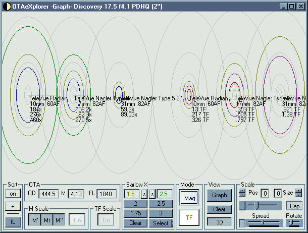
The calibration scales shown can be optionally included and are preset and not user configureable.
With all this in mind, you can see in the demo graphs that the 10mm Radian is yielding just under Mr [and a bit under M" with the 2.5x barlow] and the 31mm Nagler is nearly right-on M' [the graphset on the left is the Mag graph here].
The scale for the Mag function locates the M', Mr and M" for reference [smallest to largest ring respectively. Note that if the 'M' values have not been computed in the MPW Powers Mode section these scales will not display].
The scale for the TrueField function is calibrated in degrees at .125, .25, .5, 1, 2, 4 and 6 for reference [smallest to largest ring respectively]. Basically, each ring is a 100% increase in field of view, with the exception of the last ring (6 degrees) which is only a 50% increase from the previous 4 degree ring. Figure degrees from the inside [smallest degree: .125] out, as the larger rings can be left out of the scale for OTA/ocular configurations with maximun fields substantially less than the maximum degree calibration. The TF scale always starts with .125 degrees as the innermost ring but the outer TF scale ring, therefore, is not always representing the 6 degrees. In fact, the 4 degree and the 6 degree in particular will probably not be very often displayed.
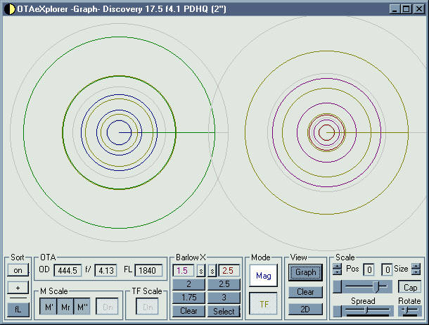
Below is a '2D' version to give a different perspective. The super-imposition shows the oculars combined steps in power and field and duplications should be readily apparent. For those interested in ocular sets to be combined with one or more barlows, with this mode you will be able to quickly identify duplicated magnification power and/or field of veiw in the various eyepiece/barlow combinations. Of course, even though not shown here, OTAeXplorer will graph up to as many as 24 eyepieces at a time.
Below is a graph of the same oculars with only the 2.5x barlow [and 'captions' turned off]. It's a combined Mag and TF '3D' graph [on the left and right respectively] with a '2D' Mag graph in the middle. As the size and placement of the graphs is adjustable, when the Graph window is set for full screen, the only limit to the number of of these types of combinations is the size of your monitor.
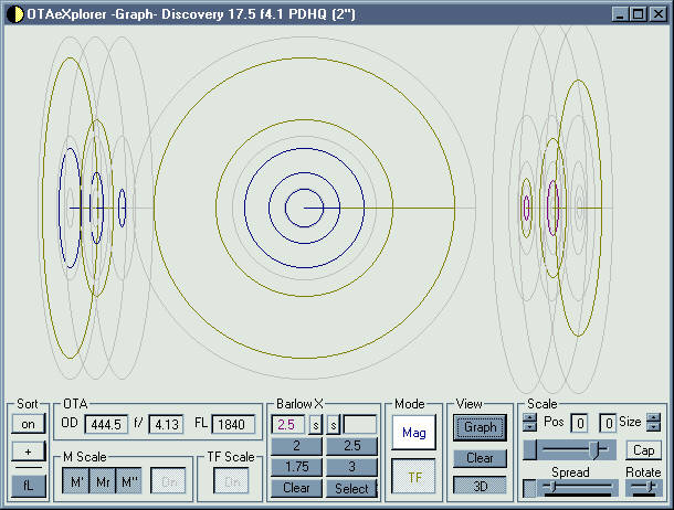
Colors of the graph display can be adjusted to some extent. The colors available however, are only those of the 16 Color VGA pallet. To change colors, the 'Set' button in the Barlow X box must be active [as shown in the above graph. Clicking on the 'Select' button will change it to 'Set' mode].
Right-clicking on the Graph button will cycle through the available color sets on the active 'Mag' or 'TF' graph. The barlow colors change along with the main color. To adjust them separately, right-click on the barlow power button just below the corresponding barlow power display box and the particular barlow color will increment.
The Power and TrueField scale colors can be altered by right-clicking on their activation buttons. The individual scale calibration rings are always displayed in the same color as a group and are not individually color-selectable.
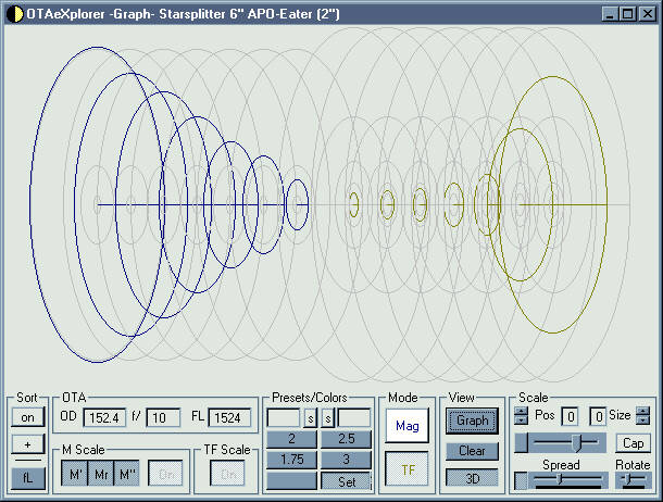 |
Here's a different OTA showing a Mag and TF graph with [from left to right, though not captioned] UO Orthos in 5mm, 6mm, 7mm, 9mm and 12.5mm with 16mm Nagler and Proxima 31mm for the two low-end powers. |
Graph color values are saved along with the other graph parameters. To restore the original default values, right-click on the viewbox 'clear' button. Default colors will then be restored to any color-change button [Mag or TF] that is active. The default color will not be restored to a button that is not 'depressed'. If you don't want to restore either of the Mag and TF colors, a right-click on the Mode box label will deselect them both and only the scale colors will be restored to default.
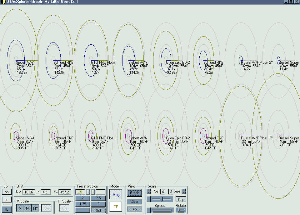
Below is some more example data of one of my own newt, EP and 2.5x Powermate setups in another graph display configuration with a full-screen (at 960x720) graph [of course you probably won't be able to fit this whole graph on your screen since it's inside the browser unless you're using at least 1024x768].
Located by the 'Size' control are two buttons, a range 'Boost' switch [the boost of which is controlled by holding down the shift, alt or control keys in any combination while activating the button and only has an effect when the 'size' value is not '0'] and a range 'Bias' control [holding the shift key down while activating this changes the direction of the bias to negative].
These have been only a few examples of the many combinations of graphs you can generate with OTAeXplorer.
In this graph, the Mag data is the top row of oculars and the TF data the bottom row:
New for OTAeXplorer [version (1.5) or later] is an additional Sort function box on the left side of the Chart and Graph control display. You can select the ocular database to be sorted in ascending (+) or descending (-) order and whether to sort by ocular focal length or field of veiw. This function can be disabled to display the oculars in the same order that they are listed in the ocular database.
The small buttons adjacent to the 'Position' and 'Spread' sliders control whether the particular slider is independant or 'ganged' between the mag and fov functions. When the button is not depressed, the mag and fov settings are independent in adjustment.
There are no sophisticated facilities built in to OTAeXplorer to print charts and graphs at this time, however, if one needs a hard-copy, most computers will print them by a press of the Print Screen button to copy the screen image to the clipboard. Using the Windows paint program or any other image editing program that has access to the Windows clipboard should then be able to send the image to your printer. 'Print Screen Deluxe' by American Systems, in particular is a very good program to use for this kind of thing and one that i can recommend. If none of these options are at your disposal, a 'Alt-rightclick' on the barlow 'clear' button will change it's function to 'Print' and a click on it in this state should send the chart or graph window being displayed to a printer.
ABOUT OTAeXplorer EYEPIECE, BARLOW AND OTA FOCUSER SIZES:
You may have noticed in the screen captures various components with descriptions 'suffixed' with 2". This is how OTAeXplorer determines compatibility between the various sizes of ocular devices.
Since 1.25" has effectively become the minimum 'standard' size for 'quality' eyepieces (with the exception of some of the smaller size orthos which are still around and may be available) and OTA's equipped with 2" focusers seeming to be ubiquitous these days, OTAeXplorer is designed to differentiate between 1.25" and 2" equipment on the ocular end of the OTA. 2.7", 4" and .965 equipment can also be specified by those corresponding designations if you wish/need to. If no size is specified in the description it is assumed to be 1.25" by default. The actual character strings OTAeXplorer looks for when determining ocular size compatibility are listed on the 'Setup' window [and the strings can be enclosed in parenthesis ( ) if you wish and they will still be recognized].
To avoid 'compatibility issues' (i.e. you can't really use a 2" eyepiece in a 1.25" focuser or barlow etc.) and having OTAeXplorer spit-out bogus chart and graph data to you, if you add the appropriate designation to the description of OTA's, eyepieces and barlows that are different than the default 1.25", OTAeXplorer should be able to figure things out correctly.
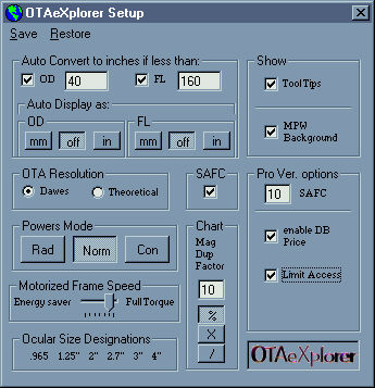 |
To change any of the Default settings use this window by clicking on the 'Setup' item under the 'Info' Menu. The change(s) will only become permanent after the 'Save' menu item at the top is clicked.
Under the 'Restore' menu item you will see options to restore the standard default values or to restore the values to the way the Main Program Window happens to be currently configured.
The database/catalog 'price' function and 'limited access mode' selectors are features of the commercial 'Pro' version. |
If you have any problems with the program or suggestions please feel free to contact me at andykidd@yahoo.com
Pricing
The Databases and Catalogs of the Pro Version have optional facilities for including item prices. You can select whether pricing is enabled or not through the 'Setup' menu.
Catalog Search
Also available in this version are Catalog Search functions which make retrieving specific item types from the catalogs virtually automatic. Tolerance ranges used in searching [including price] are adjustable and include 'less than', 'greater than' and 'about'. A right-click on the appropriate parameter label will highlight it indicating activation. A shifted right-click on the highlighted label will cycle through the search options for that parameter.
Parameters in the MPW are automatically transfered to the parameter boxes when the Search function is activated. Primary parameters [FL for oculars and OD for OTAs] are automatically selected as search parameters. Secondary parameters [AF for oculars and FL for OTAs] are enabled as search parameters by a right-click on the parameter label to highlight it.
The Search function is catalog-selective and will display a checkbox list of all pertinent catalogs in the active directory. Left-clicking a catalog will toggle the checkbox. Right-clicking the checkbox list will toggle all catalog checkboxes. Only checked catalogs are searched.
Limited Access Mode
When Limited Access Mode is enabled, permanent changes to the Catalogs and Main and Alt Databases is not allowed through the program.
Functions that are not available in this mode will either be grayed-out on the menus or will display a notification when activated. Of course enabling or disabling this mode is password protected.
Additional Chart Data
In addition to the 'Unique' and 'Duped' powers totals, the Pro 'Commercial' version will display 'Total Price' of the chart items as well as 'Cost per Magnification' of the various OTA-Ocular-Barlow combinations. OTA and Barlow prices can be selectively removed from or included in the price calculations by double-clicking the appropriate label [the label will change color to indicate it is left out of the total cost].
Non-ocular equipment such as diagonals or filters that you want to be included in the cost analysis can be included in an ocular filebase [and will be taken as 'null' except for the price] by 'prefixing' the item description with the @ character [and a space if you include an actual description i.e. @ Sirius VFS]. Of course the price field will have to have a price in it for the additional price to be included.
OTA DATABASE- One each: Main, Alt and Temp 9-array filebases.
SUMMARY OF AVAILABLE DATABASES FOR OTAs, EPs AND BARLOWs
EP AND BARLOW DATABASES- One Main, Alt and Temp 'global' 9-array bases. Additional 'OTA specific' 9-array bases of each type linked to each individual OTA in the Main, Alt and Temp OTA filebases.
to top
For those interested in the mathematics, the Amateur Astronomer's Handbook by J.B. Sidgwick (Dover Publications) elaborates on the formulas involved for these calculations
Dawes' empirical criterion for maximum resolution yields somewhat more optimistic values than theory.
Although I've never attempted to verify this, I imagine that under ideal 'seeing' conditions with high-quality optics this probably is the case.
-ak
to top